For a first encounter, follow sections 01–06. For detailed study, continue from the declared model through constraints, local motion and stability. The sources provide specific locations for further reading.
01Structure before geometric description
In FBM, structure is primitive. Geometry is a projection of structure.
This priority governs how the examples are read. First we declare the structure and relationships under examination. We then study the geometric representation and observation supported by that particular description. A shape or equation, detached from this declaration, does not suffice to determine structural identity.
Structural starting point: Constraint Theory, Axiomatic Core, Axiom 2 — Constraint Primacy. Projection and identity: Manifest §10, p. 6 ↗. The wording here is an introductory synthesis.
In the previous chapter, we examined how different declared geometric possibilities can give the same selected observation. The next question concerns the basis of that description: what must we declare to discuss a system’s possibilities?
In its account of the corpus, the Manifest connects admissibility with constraint-defined structure. It also identifies fixed reference structure, active constraint sets and admissible regions as subjects of the Theoretical Monograph.
A useful starting point for a reader is to distinguish the description of the system, the conditions declared and the states that satisfy them. The argument that follows needs to remain connected to that declaration.
Basis for the discussion: Corpus Manifest v1.0, §§1–2, p. 2 · §3.1, pp. 2–3 ↗
02What do we declare before analysis?
The term “fixed reference structure” asks us to identify the structure to which the analysis refers. The Manifest locates the concept within the corpus; its full development belongs to the Theoretical Monograph. Here, we organise an introductory reading around four questions:
| Element of the description | A question to answer |
|---|---|
| System and reference structure | Which system are we examining, and which reference structure do we declare for its description? |
| Constraints and conditions | Which relations must hold, under which declared conditions? |
| Variables and domain | Which quantities describe a state, and which values are considered? |
| Projection and observation | Which map connects the description to the observed quantity, and which distinctions does it permit? |
This table helps organise the discussion. It helps us recognise, for example, when a claim refers to a particular set of conditions and when those conditions have changed without being declared.
The Mathematical Monograph develops the corpus’s formal objects. The triangle below is a standalone mathematical aid for conditions holding simultaneously. Its construction does not declare a complete FBM structural object and its projection rule. In the later rod, pivot and guide example, the mechanical arrangement is declared before its geometric equations.
Basis for the discussion: Corpus Manifest v1.0, §§3.1–3.2, pp. 2–3 ↗
03The conditions are considered together
Let us describe a geometric state using two dimensionless coordinates, x and y, each between 0 and 1. We declare two conditions: y must be at least as large as x, and their sum must not exceed 1.
C1: y ≥ x
C2: x + y ≤ 1
A state is admissible in this example when it satisfies both conditions simultaneously within the declared domain. The set of all such states forms a triangular region. Because the inequalities permit equality, its boundaries are included.
Point P = (0.25, 0.50) satisfies both conditions. Q = (0.40, 0.80) satisfies the first but violates the second: 0.40 + 0.80 = 1.20. Satisfying one condition alone is insufficient for a point to belong to the common region.
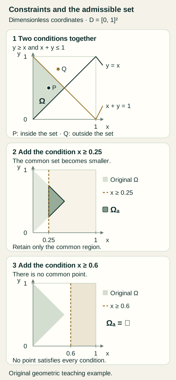
An original geometric example for the chapter, with local notation. It does not reproduce the formal FBM definitions or experimental results.
04What changes with an additional constraint?
We retain the same domain and the two original conditions. We now add the requirement x ≥ a, where a is a declared parameter between 0 and 1. The new condition retains only the points of the original region on or to the right of the corresponding vertical line.
| Parameter a | What remains |
|---|---|
| 0 | The original triangular region: the additional condition already holds throughout the declared domain. |
| 0.25 | A smaller triangular region, with all conditions holding simultaneously. |
| 0.50 | A single point: (0.50, 0.50). |
| 0.60 | The empty set: no point satisfies all conditions. |
Here we change the declared geometric requirement. For this family of examples, increasing a makes the remaining set smaller or leaves it unchanged. A single remaining point and an empty set are different outcomes.
The mathematical development of the example
We define the domain D = [0, 1]2 and use the following local notation:
Ω = { (x, y) ∈ D : y ≥ x, x + y ≤ 1 }
Ωa = { (x, y) ∈ Ω : x ≥ a }
The two original inequalities give x ≤ y ≤ 1 − x. Thus x ≤ 1/2 is required. With the additional constraint, we need a ≤ x ≤ 1/2.
For 0 ≤ a < 1/2, Ωa is the triangle with vertices (a, a), (a, 1 − a) and (1/2, 1/2). At a = 1/2 the vertices coincide and a single point remains. For a > 1/2 there is no common solution.
If 0 ≤ a ≤ b ≤ 1, then Ωb ⊆ Ωa. Adding a condition that must hold together with the preceding ones retains or excludes states; it introduces no new states in this construction.
These relations describe only this example. They do not define a trajectory, forces, equilibrium or a criterion for physical validation.
An original geometric example for the chapter, with local notation. It does not reproduce the formal FBM definitions or experimental results.
05One admissible state does not describe the whole set
Point P = (0.25, 0.50) remains admissible both in the original region and after adding x ≥ 0.25. A record of that point would agree with both descriptions.
The descriptions nevertheless permit different possibilities: for example, (0.10, 0.50) belongs to the original region and is excluded by the additional condition. This connects the present example to the question of a mechanical trace: an observed state can be compatible with more than one declared set of possibilities.
The observation’s inability to distinguish these two descriptions does not cancel its information. It identifies how far that information can support an interpretation without further evidence.
Basis for the discussion: Corpus Manifest v1.0, §10, p. 6 ↗ — compatibility / attribution distinction. The specific points and sets belong to the original example.
06The scope of admissibility in this example
In our construction, “admissible” means that a point belongs to the set defined by the declared geometric conditions. To discuss a physical mechanism’s behaviour, we would also need to examine the additional relations and evidence required by the particular claim.
The example does not select which state will be realised, which path will be followed or whether a state will be stable. Even the single point at a = 0.50 is a result of the inequalities, without physical equilibrium or stability having been established.
Likewise, the empty set at a = 0.60 shows incompatibility of these particular conditions within this particular domain. It does not by itself establish that no physical system can function under a different description.
This distinction connects to the Manifest’s requirement to separate internal validation from agreement with physical reality and to support each claim with appropriate evidence.
Basis for the discussion: Corpus Manifest v1.0, §3.2, p. 3 · §10, p. 6 · §§12–13, p. 7 ↗
07Representing a declared arrangement
In the mechanical example, we first declare an ideal rigid rod and fixed pivot; we then add a bilateral guide. Rigidity, connections and imposed conditions are data of the idealised arrangement. We subsequently choose coordinates and write relations expressing the geometric consequences of those data.
Sections 07–12 use classical mathematical tools to analyse particular declared models. Their relationship to complete FBM structural definitions is examined through the comparison questions in section 13.
For this selected representation, use the following local notation. Let q = (q1, …, qn) be coordinates in an open region U ⊂ ℝn. They describe a configuration: the geometric arrangement under examination. If velocities are also needed to predict evolution, q alone is not a complete dynamical state.
Collect into a parameter λ what we hold fixed in each analysis: lengths, guide positions or other declared settings. Write the conditions as equalities and inequalities, using a consistent sign convention:
hi(q; λ) = 0, i = 1, …, m
gj(q; λ) ≥ 0, j = 1, …, k
Qλ = { q ∈ U : h(q; λ) = 0, g(q; λ) ≥ 0 }
Here Qλ is the model’s admissible set: the common solution of the declared conditions. Inequalities are interpreted componentwise. This notation is local to the chapter. It lets us examine separately a change in coordinates q, a change in parameter λ, and replacement of the relations h, g themselves.
The variables also determine which information the model retains. For example, a rod endpoint position does not by itself describe elastic deformation of the rod. Choosing rigid bodies is an assumption that needs to suit the question and the evidence of the study.
Related established terminology: configuration space, Lynch & Park, Modern Robotics, Definition 2.1, p. 12. Qλ and the organisation of parameters are the declared construction of this development.
08What does a constraint permit to first order?
Begin with smooth equalities only, holding λ fixed. If a differentiable curve q(s) remains admissible, then h(q(s); λ) = 0 for every s. The chain rule gives:
Jh(q; λ) q′(s) = 0
(Jh)ij = ∂hi / ∂qj
The constraint Jacobian Jh collects derivatives of the constraints. Every tangent to an admissible curve belongs to its kernel. Here s is the curve parameter; when it is time, q′ is the configuration velocity. This matrix concerns constraints. A Jacobian mapping joint velocities to an endpoint velocity serves a different role.
At an admissible point q0 with h(q0; λ) = 0, if the m equalities are independent, meaning rank Jh = m, the implicit function theorem gives a local smooth configuration set of dimension n − m. Its tangent space is the kernel of Jh. More generally, constant rank r on an open neighbourhood gives the corresponding local dimension n − r. Constancy of rank is an essential assumption.
For the endpoint of an ideal rigid rod of length L > 0, with its other end pivoted at O = (0, 0), we have x² + y² = L². The Jacobian is the row (2x, 2y), of rank 1 everywhere on the circle. At (L, 0), the relation 2Lx′ = 0 permits vertical tangents. One admissible curve is q(s) = (L cos s, L sin s).
The algebraic formula dim ker J = n − rank J holds for every matrix. Interpreting it as actual local mobility requires the geometric assumptions just stated. The next example shows what happens when they fail.
Connection to closed-chain mechanics: Modern Robotics, §7.3, pp. 256–258. The differentiation and rod example are developed here for the specific declared idealised arrangement.
09When linearisation leaves extra possibilities
Add an ideal horizontal guide at the endpoint of the same rod, imposing y = a. The guide is bilateral: the endpoint stays on the line. The quantities x, y, L and a have the same unit of length. Take a ≥ 0 and hold a fixed in each analysis.
The rod, pivot and guide form the declared idealised arrangement. The circle and line represent its constraints geometrically in the selected coordinates.
The question is which endpoint positions are compatible with these connections, with L and a fixed. Geometry lets us answer exactly. The role of the bilateral guide becomes explicit in the comparison with a unilateral constraint, where the imposed relation changes.
Fa(x, y) = (x² + y² − L², y − a) = (0, 0)
x² = L² − a², y = a
| Guide position | Exact solutions | Rank of Ja at the solutions |
|---|---|---|
| 0 ≤ a < L | Two points: (±√(L² − a²), a) | 2 at each point |
| a = L | One point: p = (0, L) | 1 |
| a > L | No solution | No admissible point at which to evaluate |
Admissible rod endpoint positions
Lengths are expressed in units of L, with L = 1 in this figure. The constraints are x² + y² = 1 and y = α, where α = a/L.
We vary a geometric parameter, not time. The figure compares admissible configurations for different guide positions; it does not simulate dynamics or motion within a fixed admissible set.
The rows of Ja are (2x, 2y) and (0, 1), so det Ja = 2x. At both points with a < L, the kernel is zero: each point is isolated and no continuous motion connects them while the guide remains fixed.
At the tangent position a = L, the matrix loses rank. The linear condition gives only y′ = 0, leaving x′ apparently free. Yet the full equations have only the solution (0, L). No nonconstant admissible curve passes through it with the guide in that same position.
The next derivative reveals the limitation
For a twice differentiable admissible curve, y = L gives y′ = y″ = 0. Differentiating the circle equation twice gives:
2(x′)² + 2(y′)² + 2xx″ + 2yy″ = 0
At p = (0, L): 2(x′)² = 0, hence x′ = 0.
Second order excludes the nonzero horizontal tangents allowed by first order. Solving the equations exactly already proves the stronger result: the admissible set contains just one point.
Here rank loss concerns this particular constraint representation. The same singleton can be described by x = 0 and y = L with a full-rank Jacobian. Thus 2 − rank Ja = 1 at p measures the linearised kernel of these equations; it does not establish one actual degree of freedom.
What changes if the guide is allowed to move as well?
The question changes and a variable is added. The curve x(s) = L sin s, y(s) = a(s) = L cos s satisfies both relations and has a horizontal tangent at s = 0. It does not belong to the set with a fixed at L. The distinction between a parameter and a variable determines the conclusion.
Furthermore, solution sets for different values of a lie on different horizontal lines. They do not form the nested family of the preceding triangular example.
An original idealised mechanical example with an exact geometric representation. It examines admissible positions and the linearisation of declared constraints, without introducing forces or representing a particular articulator.
10An active constraint and one-sided possibilities
An inequality g(q) ≥ 0 is called active at a point when g(q) = 0 there. This does not require it to remain an equality during the next admissible change. The change can point into the region’s interior.
The same recorded position, different possibilities
Return to the rod with its fixed pivot. Keep the same length L, coordinates and height a = 3L/5. Change only how the endpoint is constrained: compare the bilateral guide with an ideal unilateral constraint imposing y ≥ a. The latter declaration concerns the endpoint position only.
| Declared relation | Geometric consequence |
|---|---|
| Bilateral guide: y = 3L/5 | The endpoint retains the same height. Together with x² + y² = L², this leaves two isolated positions: (±4L/5, 3L/5). |
| Unilateral constraint: y ≥ 3L/5 | The endpoint may move towards larger y. The entire closed upper arc of the circle with y ≥ 3L/5 remains, including both endpoints. |
Position P = (4L/5, 3L/5) is admissible in both descriptions. A record of that position alone does not reveal which relation holds. The interactive figure in the preceding section calculates the bilateral-guide case.
An admissible curve that distinguishes the two declarations
Set θ0 = arcsin(3/5) and, for sufficiently small s ≥ 0, write:
q(s) = (L cos(θ0 + s), L sin(θ0 + s))
q(0) = P, q′(0) = (−3L/5, 4L/5)
The curve remains exactly on the circle and, for sufficiently small s > 0, has y(s) > 3L/5. It is therefore permitted by the unilateral condition and excluded by the bilateral guide. Here s is a curve parameter; no time law or force realising this motion has been specified.
Geometry does essential work here: it calculates and distinguishes the possibilities implied by the two declared relations. The circle, the line y = a and position P can appear in both descriptions, while the full admissible set differs. To obtain this result, we must first know whether the endpoint is retained on the boundary or may move away from it.
An original comparison of two idealised declarations within the same example. The solutions follow from the equations given here. No canonical FBM regime definition or conclusion about contact forces is introduced.
An active inequality permits departure from the boundary
At P, the inequality g(x,y) = y − 3L/5 ≥ 0 is active. For a one-sided admissible curve, the rod requires 4vx + 3vy = 0 and the unilateral constraint requires vy ≥ 0. The admissible tangents are the nonnegative multiples of (−3, 4): they form a tangent cone, here a ray. The curve above, its reparameterisations and the constant curve realise these tangents.
With the bilateral guide, vy = 0 is additionally required, hence vx = 0 as well. The directional difference follows from the change in the imposed relation, with L and a unchanged.
In general, for differentiable inequalities, every velocity of a one-sided admissible curve satisfies ∇gj(q) · v ≥ 0 at active constraints, alongside the corresponding equality conditions. This condition is necessary. Its sufficiency requires further examination in the general nonlinear case; here the explicit admissible curves establish the description.
For ideal contact, geometric nonpenetration is only one part of the description. Reaction force and contact relations are examined separately in the chapter on mechanical regimes.
11Coordinates, parameters and velocity constraints
The same geometry in different coordinates
If q = φ(z) is a smooth local coordinate change with a smooth inverse, the same constraints become h(φ(z); λ) = 0. The chain rule gives Jz = JqDφ. Since Dφ is invertible, rank is preserved and tangents map between the two descriptions.
In the rod example, set u = x and v = y − a, with a fixed. The guide becomes v = 0, but the circle becomes u² + (v + a)² = L². The parameter remains in the geometry. Translating the coordinate origin does not move the guide relative to the pivot.
When does a velocity relation introduce a different kind of condition?
A holonomic constraint can be expressed as a relation among configuration coordinates; here we consider relations without explicit time dependence. Differentiating it produces a velocity relation A(q)q̇ = 0. Writing a condition in this form is not enough to call it nonholonomic: it must not be locally replaceable by equivalent configuration-only constraints.
An ideal vehicle rolling without lateral slip, with position (x, y) and orientation θ, satisfies:
sin θ · ẋ − cos θ · ẏ = 0
The relation excludes an immediate lateral velocity at the current θ. Successive manoeuvres can nevertheless produce a net lateral displacement. Instantaneously admissible velocity and configurations reached through a path are therefore different objects of study.
For holonomic / nonholonomic constraints and the ideal vehicle: Lynch & Park, official companion material §2.4. The coordinate change for the example is calculated here.
12From admissibility to equilibrium and stability
To examine what dynamics adds, now declare a different, complete example: a dimensionless scalar state z ∈ ℝ and dimensionless time τ ≥ 0, with initial condition z(0) = z0. Compare two evolution laws on the same state set:
System A: dz/dτ = −z, z(τ) = z0e−τ
System B: dz/dτ = +z, z(τ) = z0eτ
In both, z = 0 is an equilibrium: starting exactly there means remaining there. In A, every initial deviation decreases exponentially. In B, every nonzero initial deviation increases exponentially. A shared state set and equilibrium position coexist with different stability.
Lyapunov stability requires that, for any prescribed small neighbourhood of the equilibrium, all future states remain within it when they start sufficiently close. Asymptotic stability additionally requires convergence to the equilibrium. In A, |z(τ)| ≤ |z0| and z(τ) → 0 as τ → ∞. In B, for any nonzero z0 and any fixed bound ε > |z0|, |z(τ)| eventually exceeds ε.
This example shows that a shared state set and equilibrium position do not determine dynamical stability. The comparison concerns the two declared evolution laws and the Lyapunov criterion. Using stability in a particular FBM study requires the definition and assumptions of that source.
Equilibrium and stability terminology: Tedrake, Underactuated Robotics, “The Simple Pendulum”, section “The overdamped pendulum”. The comparison of the two exponential solutions is an original example for this chapter.
14Connecting theory, mathematics and the Atlas
The theoretical route raises the questions of declared structure, admissibility and the organisation of constraints. The mathematical route develops the relevant objects and their relationships, alongside interaction, equilibrium and stability.
The Atlas contributes the specific empirical domain of articulators: traces, dominance distribution, contact continuity, friction and structural validation. Connecting these subjects requires reading each result together with its declared conditions and relevant evidence.
Our geometric example offers a first tool for understanding constraints that hold together. Active constraints, dominance and mechanical regimes require their own conceptual development. A change in the shaded set is not automatically classified as a mechanical regime transition.
To assess a claim about admissibility, we need to know which system is described, which conditions are declared and which evidence connects the description to the subject of the study.
Basis for the discussion: Corpus Manifest v1.0, §§3.1–3.3, pp. 2–3 · §13, p. 7 ↗
The study of partial adjustability offers a concrete question for this method: which change concerns a setting parameter, and which changes the arrangement of constraints? The theoretical note on the Hanau H lets us continue from an admissible set to the particular equilibrium selection declared in that source. Connecting with actual records requires the geometry, contact conditions and measurements of the arrangement under examination.
15Sources and further reading
This chapter combines introductory synthesis with original mathematical development. The place of concepts in the corpus is documented through Manifest v1.0, with sections and pages beside the relevant claims. The rod, inequalities, derivatives and dynamical examples are developed here from their declared equations. Related literature provides specific points of comparison. The full formal definitions of FBM belong to the corresponding monographs.
- Theoretical Monograph — reference structure, constraints and regimes ↗
- Mathematical Monograph — objects, admissible sets and relationships ↗
- Atlas Monograph — the empirical articulator domain ↗
Locators use the preprint’s printed pagination: Definition 2.1, p. 12; §2.4, pp. 30–31; §7.3, pp. 256–258. These page numbers are not attributed to the 2017 printed edition.
Locators: holonomic and Pfaffian constraints; the car example of a nonholonomic constraint.
Locators: definitions of fixed point, local Lyapunov stability, and asymptotic stability. Accessed 19 October 2026.